Firstly, it feels good to blog again after a seven year hiatus. Secondly, starting with this post, I am starting a series on Efficient AI techniques (architecture, optimization, data, etc.). Most of these posts are going to be focused on techniques for improving autoregressive decoder-only models (LLMs) while also being generally applicable to other models with some tweaks. I also assume that you are familiar with the basics of the transformer architecture (if you are not, this or this might be good first steps.).

Summary

Doing inference on transformers can be expensive. Inference latency scales linearly with the model depth / number of layers ($l$) in the model. Efforts like Early Exits aim to reduce the number of layers used while processing easier tokens (for some definition of ‘easier’), but aren’t trivial to implement. We will cover it in a future post.

In this post, we cover two different, but related techniques:

1. KV Caching: cache and reuse the K, V representations of tokens that are already computed in previous steps. You might already be familiar with his.
2. KV Sharing: share the key and value representations ($K$ and $V$) of tokens across the last half of the layers of a transformer model. Therefore avoiding re-computing them across the last half of the layers. Other weight tensors such as query, MLP, etc. remain non-shared. This is a relatively newer technique.

Discussion

One of the reasons for a naive transformer implemention’s expensive inference is the need to compute the key, and value representations for all the tokens in the given sequence in the Self-Attention module. It looks something like the figure below.

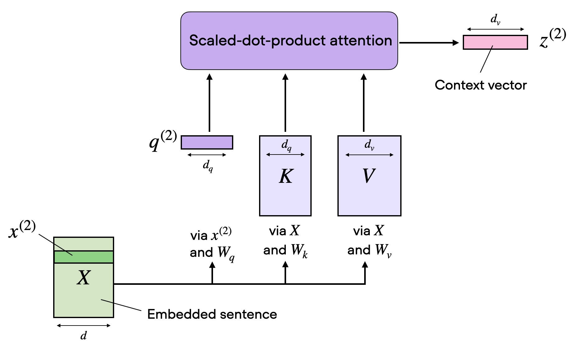
A typical Self-Attention block. Source: Sebastian Raschka's blog.

Since transformers are typically operating in the auto-regressive (AR) setting, this works as follows:

1. Assume we have a sequence of tokens $S = [s_0, s_1, s_2, …, s_{n-1}]$, that we have already generated.
2. To predict the next token, $s_n$, we need the K, V representations of all the tokens in the sequence seen so far. And we need to do this for the $l$ layers.
3. This means we need to compute $l$ matrices of size $(n-1) \times d$, where $d$ is the model dimension / embedding dimension, via a matrix multiplication of the form $X . W_i$, where $X$ is the input at a particular layer, and $W$ is either the key or value weight matrix ($W_K$ or $W_V$) at that layer.
4. This is expensive because we will incur $l$ matrix multiplications, each costing $O(nd^2)$, for a total cost of $O(lnd^2)$ per predicted token! It’s growing faster than the US National Debt!

In the above calculation, we assume a single attention head. Thus the total cost of computing the K,V representations per head ($O(lnd^2)$) is made up of three components:

1. Sequence Dimension: The number of tokens seen so far ($n-1$).
2. Depth Dimension: The number of layers ($l$).
3. Model Dimension: The width of the input stream ($d$).

We can’t do much about $d$ yet, but let’s see how we can tackle the other two for now.

1. KV Caching: Optimizing the sequence dimension.

KV Caching suggests there are two things happening during inference:

• Model weights, including $W_K$ and $W_V$ are fixed.
• K, V representations for a given token $s_i$ only depends on that token and $W_K$ and $W_V$.

Since $W_K$ and $W_V$ are fixed, once we compute the K, V representations for a given (token, layer, head) tuple, it can be reused when predicted any subsequent tokens by caching those representations in memory and reusing them for the next step.

If we can do this, we would only need to compute the K, V representations of the $s_{n-1}$ token when predicting the $n$-th token, since that’s the only token for which we don’t have the K, V vectors. Therefore, it is easy to show that the new total cost of computing the representations is $O(ld^2)$, an $n$-times speedup! This is a significant win, especially if the sequence is very long.

Question: Why don’t we cache the query representation?
Answer: We only compute and use the Q vector of the last token in the Self-Attention block. Thus, there is no need for caching the Q representations for the previous tokens.

2. KV Sharing: Optimizing the depth dimension.

KV Sharing reduces the cost of computing the K, V representations in the depth-dimension ($l$). Concretely, the proposal is that the actual K, V representations are the same between the last half (or any other fraction) of the layers.

Note that we are referring to the actual $K$, $V$ tensors being the same, not just the $W_K$ and $W_V$ matrices being shared. What this means is that the last layer which doesn’t share the K, V representations computes them once, and they are used as is across the remaining half of the layers (regardless of what the inputs are to these layers).

Said in an even simpler way, there is a KV cache across the last half of the layers. This is illustrated in the figure below.

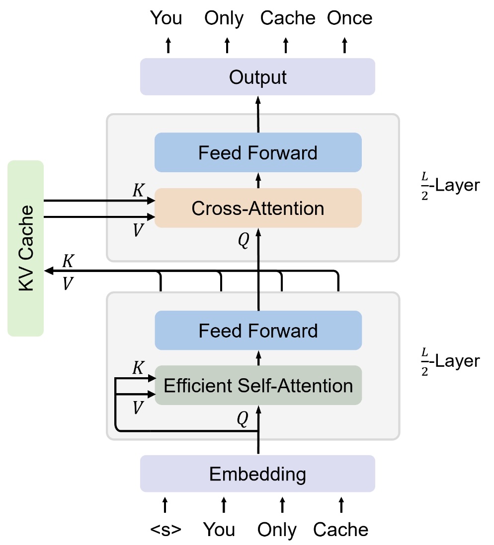
KV Sharing. Source: You Only Cache Once paper.

The figure above illustrates the KV Sharing by showing a shared KV cache between the last $l/2$ layers. It is easy to see that if this works, we can simply not compute the K, V representations for $l/2$ of the layers. More generally, we save $l/k$ of the FLOPS, if the last $l/k$ layers are shared.

However, to make this work we need to ensure that the model is trained with the KV-Sharing behavior. This is detailed in the You Only Cache Once paper.

Some of the intuition behind why this even works in the first place, comes from works like these, which show empirically that in a deep transformer-like model, the last layers are correlated with each other. What this means is that the last few layers are not necessarily adding a lot of new information, but just tweaking the output so far. This redundancy can potentially be exploited (on another note, how can we make these layers do more heavy lifting?).

Additionally, note that we are only sharing the K, V representations, so it only affects the representations of the tokens seen in the past in the Self-Attention block, and is allowing cheap some degrees of freedom to the model.

Another bonus of this technique:

1. You also save a lot of memory, since you don’t have to store $W_K$ and $W_V$ at all.
2. It is applicable during training as well, so you save on inference and memory during training too.

Conclusion

In this post we saw that we can significantly reduce the costs associated with computing the K,V representations in the Self-Attention block using KV Caching and KV Sharing. Concretely, we reduced it by a factor of:

1. $n$ by implementing KV Caching.
2. $l/2$ by implementing KV Sharing across the last $l/2$ layers.

The total cost is now $O(ld^2)$, but with a significantly smaller constant due to KV Sharing. Additionally, KV Sharing eliminates the $W_K$ and $W_V$ matrices for half the layers, which is another huge gain.

That brings us to a the end of this post. Please feel free to drop in any comments if I missed something.