Scaling SGD

01 Apr 2018 - 3 minute read

I’ve been reading a few papers related to scaling Stochastic Gradient Descent for large datasets, and wanted to summarize them here.

Large Scale Distributed Deep Networks - Dean et al., 2012 [Link]

One of the popular papers in this domain, talks about work on a new distributed training framework called DistBelief. Pre-cursor to the distributed training support in Tensorflow.
Before this work, ideas for doing SGD in a distributed setting restricted the kind of models (convex / sparse gradient updates / smaller models on GPUs with gradient averaging).
This works describes how to do distributed asynchronous SGD.

Model-Level Parallelism: Works with large models by splitting the model graph itself into several parts. Each part of the model is assigned to a different machine. If there is an edge between two nodes in different parts, the two machines hosting those parts would need to communicate. This is to get around the problem of fitting a large model on a single GPU.

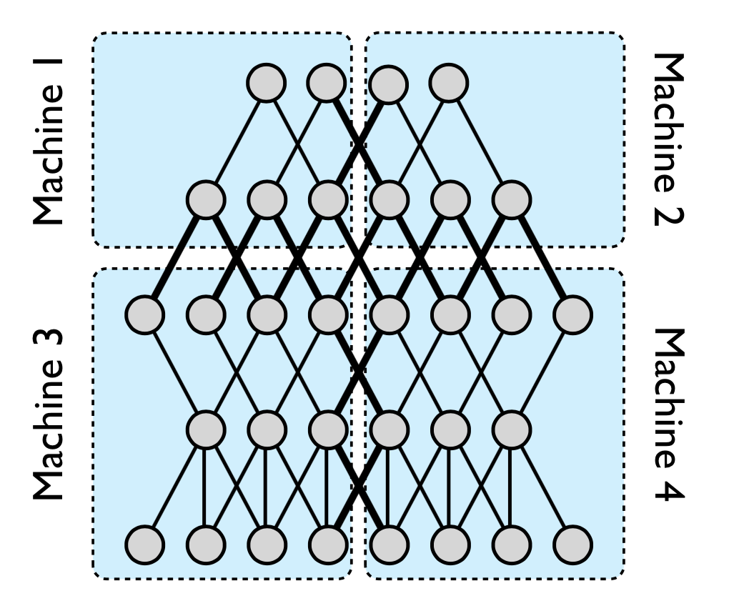
Figure 2: Splitting the Model Graph.

Downpour SGD: To be able to scale to large datasets, DistBelief also runs several replicas of the model itself. The training data is split into several subsets, and each replica works on a single subset. Each of the replica sends the updates of its params to a Parameter Server. The parameter server itself is sharded, and is responsible for getting updates for a subset of params.

Whenever a new replica starts a new minibatch, it gets the relevant params from the parameter server shards, and then sends its updates when its done with its minibatch.

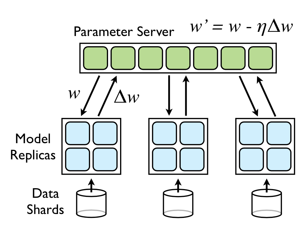
Figure 2: Parameter Server.

The authors found Adagrad to be useful in the asynchrous SGD setting, since it uses an adaptive learning rate for each parameter, which makes it easy to implement locally per parameter shard.

Accurate, Large Minibatch SGD: Training ImageNet in 1 Hour - Goyal et al. (2017) [Link]

This paper describes how the authors trained ImageNet using synchronous SGD. However, given the synchronous nature of SGD, the idea is to use large batches (of the order of thousands of samples), instead of mini-batches (which are typically in the tens of samples), to avoid the communication overhead.
They demonstrate that with their method, they are able to use large batch sizes (up to 8192) without hurting accuracy with a ResNet-50 model (as compared to the baseline model with a batch-size of 256). Using 256 Tesla P100 GPUs, their model trains on the ImageNet dataset within 1 hour.
Linear Scaling Rule for Learning Rate: “When the minibatch size is multiplied by $k$, multiply the learning rate by $k$.”. One way to think about this is, if the batch size is increased by $k$ times, there are $k$ times fewer updates to weights (since there $k$ times fewer iterations per epoch). Another intuition is, with smaller batches the stochasticity (randomness) of the gradient is higher. With bigger batches, you can confidently take bigger steps.
The authors do a gradual warm-up of the learning rate from a small value, to the target learning rate, per the linear scaling rule. The authors hypothesize that the linear scaling rule breaks down for large batches in the initial stages of the training, where a gradual warm-up helps with better training.

ImageNet Training in Minutes - You et al. (2018) [Link]

Another paper that is similar to the paper by Goyal et al. They use a bigger batch-size (32k instead of 8k).
As per the numbers reported in the paper, with a 32k batch size, they get accuracy comparable to smaller batches. The training finishes in 14 minutes using unspecified number of Intel Knights Landing CPUs (possibly 1024 or 2048).
They use the gradual warm-up reported in Goyal et al., along with an algorithm that tweaks the learning-rate on a layer-wise basis (LARS algorithm - You et al., 2017). The LARS algorithm is similar to Adagrad (which works on a per-param level), which was useful in Dean et al.’s work.

Dynamic Programming: You Can Do It Half Asleep!

16 Aug 2017 - 5 minute read

That was a click-baity title. :)

But seriously, people make a big deal out of ‘Dynamic Programming’, in the context of software engineering interviews. Also, the name sounds fancy but for most problems in such interviews, you can go from a naive recursive solution to an efficient solution, pretty easily.

Any problem that has the following properties can be solved with Dynamic Programming:

Overlapping sub-problems: When you might need the solution to the sub-problems again.
Optimal substructure: Optimizing the sub-problems can help you get the optimal solution to the bigger problem.

You just have to do two things here:

Check if you can apply the above criteria.
Get a recursive solution to the problem.

That’s it.

Usually the second part is harder. After that, it is like clockwork, and the steps remain the same almost all the time.

Example

Assume, your recursive solution to say, compute the n-th fibonacci number, is:

\[F(n) = F(n - 1) + F(n - 2)\] \[F(0) = F(1) = 1\]

Step 1: Write this as a recursive solution first

int fib(int n) {
  if (n == 0 || n == 1) {
    return 1;
  } else {
    return fib(n-1) + fib(n-2);
  }
}

Now, this is an exponential time solution. Most of the inefficiency comes in because we recompute the solutions again and again. Draw the recursion tree as an exercise, and convince yourself that this is true.

Also, when you do this, you at least get a naive solution out of the way. The interviewer at least knows that you can solve the problem (perhaps, not efficiently, yet).

Step 2: Let’s just simply cache everything

Store every value ever computed.

int cache[20];
int fib(int n) {
  // Pre-fill all the values of cache as -1.
  memset(cache, -1, sizeof(cache)); 
  return fibDP(n);
}

int fibDP(int n) {
  // Check if we have already computed this value before.
  if (cache[n] != -1) {
    // Yes, we have. Return that.
    return cache[n];
  }
  
  // This part is just identical to the solution before.
  // Just make sure that we store the value in the cache after computing
  if (n == 0 || n == 1) {
    cache[n] = 1;
  } else {
    cache[n] = fibDP(n-1) + fibDP(n-2);
  }
  
  return cache[n]; 
}

Let us compute how many unique calls can we make to fibDP?

There is one parameter, n.
Hence, n unique values of n can be passed to fibDP.
Hence, n unique calls.

Now, realize two things:

We would never compute the value of the function twice for the same value, ever.
- So, given $n$, we would call the function $n$ times, as seen above.
- Each time with $O(1)$ work in each function call.
- Total = $n$ calls with $O(1)$ work each => $O(n)$ total time complexity.
We are using up extra space.
- We use as much extra space as:
- Number of possible unique calls to the recursive function * space required for each value.
- Since there are $n$ unique calls possible with an int value, space would be $O(n)$.
- I have hard-coded a limit of 20 in my code. We can also use a Vector etc.

That’s it. We just optimized the recursive code from a $O(2^n)$ time complexity, $O(n)$ space complexity (recursive call stack space) to an $O(n)$ time, $O(n)$ space (recursive + extra space).

Example with a higher number of parameters

int foo(int n, int m) {
  if (n <= 0 || m <= 0) {
   return 1;
  }
    
  return foo(n-1, m) + foo(n, m-1) + foo(n-1, m-1);
}

Time complexity: $O(3^{n+m})$ [Work it out on paper, why this would be the complexity, if you are not sure.]

DP Code

int cache[100][100];
int foo(int n, int m) {
  memset(cache, -1, sizeof(cache));
  return fooDP(n, m);
}

int fooDP(int n, int m) {
  if (n <= 0 || m <= 0) {
   return 1;
  }
  
  if (cache[n][m] == -1) {
    cache[n][m] = fooDP(n-1, m) + fooDP(n, m-1) + fooDP(n-1, m-1);
  }
  return cache[n][m];
}

Number of unique calls: $O(nm)$
Space Complexity: $O(nm)$
Time Complexity: $O(nm)$

Assume I tweak foo and add an $O(n \log m)$ work inside each call, that would just be multiplied for the time complexity, i.e.,

Time complexity = O(unique calls) * O(work-per-call)

\[\implies O(nm) \times O(n \log m)\] \[\implies O(n^2 m \log m)\]

$Space Complexity = O(unique calls) * O(space per call)

\[\implies O(nm) \times O(1)\] \[\implies O(nm)\]

Now just reinforce these ideas with this question

Given a rectangular grid of size N x M,
What is the length of the longest path from bottom-left corner (0, 0) to top-right corner (N - 1, M - 1), assuming you can go up, right, diagonally?

Extra Credit

What we saw is called top-down DP, because we are taking a bigger problem, breaking it down into sub-problems and solving them first. This is basically recursion with memoization (we ‘memoize’ (fancy word for caching) the solutions of the sub-problems).

When you absolutely, totally nail the recursive solution, some interviewers might want a solution without recursion. Or, probably want to optimize the space complexity even further (which is not often possible in the recursive case). In this case, we want a bottom-up DP, which is slightly complicated. It starts by solving the smallest problems iteratively, and builds the solution to bigger problems from that.

Only if you have time, go in this area. Otherwise, even if you mention to the interviewer that you know there is something called bottom-up DP which can be used to do this iteratively, they should be at least somewhat okay. I did a short blog-post on converting a top-down DP to a bottom-up DP if it sounds interesting.

Back to Basics: Reservoir Sampling

30 Jul 2017 - 3 minute read

If you have a dataset that is either too large to fit in memory, or new data is being added to it on an ongoing basis (effetively we don’t know its size), there will be the need to have algorithms, which have a:

Space Complexity that is independent of the size of the dataset, and,
Time Complexity per item of the dataset that is either constant, or otherwise is very small.

Examples of such datasets could be clicks on Google.com, friend requests on Facebook.com, etc.

One simple problem that could be posed with such datasets is:

Pick a random element from the given dataset, ensuring that the likelihood of picking any element is the same.

Of course, it is trivial to solve if we know the size of your dataset. We can simply pick a random number in $(0, n-1)$ ($n$ being the size of your dataset). And index to that element in your dataset. That is of course not possible with a stream, where we don’t know $n$.

Reservoir Sampling does this pretty elegantly for a stream $S$:

sample, len := null, 0
while !(S.Done()):
  x := S.Next()
  len = len + 1
  if (Rand(len) == 0):
    sample = x
return sample

The idea is simple. Every new element you encounter, replace your current choice with this new element with a probability of $\large\frac{1}{l}$. Where $l$ is the total length of the stream (including this element), encountered so far. When the stream ends, you return the element that you had picked at the end.

However, we need to make sure that the probability of each element being picked is the same. Let’s do a rough sketch:

When the length of the stream is $1$, the probability of the first element being picked is $1.0$ (trivial to check this).
Assuming that if this idea works for a stream of size $l$, we can prove that it works for a stream of size $l+1$.
- Since it holds for a stream of size $l$, all elements before the $l+1$-th element have the same likelihood, i.e., $\large\frac{1}{l}$.
- The new element will replace the selected element with a probability of $\large\frac{1}{l+1}$, but the existing element will remain with a probability of $\large\frac{l}{l+1}$.
- Hence the probability of each of the elements seen so far being selected will be, $\large\frac{1}{l} . \large\frac{l}{l+1} = \large\frac{1}{l+1}$.
- The probability of the new element being selected, as we stated earlier is $\large\frac{1}{l+1}$.
- Hence, the probability will be the same for all the elements, assuming it holds for a stream of size $l$.
Given that the property holds for $n = 1$, and (2) is true, we can prove by induction that this property holds for all $n \gt 1$.

There could be a weighted variant of this problem. Where, each element has an associated weight with it. At the end, the probability of an item $i$ being selected should be $\large\frac{w_i}{W}$. Where, $w_i$ is the weight of the $i$-th element, and $W$ is the sum of the weights of all the elements.

It is straight-forward to extend our algorithm to respect the weights of the elements:

Instead of len, keep W.
Increment W by $w_i$ instead of just incrementing it by 1.
The new element replaces the existing element with a probability of $\large\frac{w_i}{W}$.

In a manner similar to the proof above, we can show that this algorithm will also respect the condition that we imposed on it. Infact the previous algorithm is a special case of this one, with all $w_i = 1$.

Credits:

[1] Jeff Erickson’s notes on streaming algorithms for the general idea about streaming algorithms.

Newer Older