Gaurav's Blog
Paper: Neural Graph Machines
08 Jun 2017 - 2 minute read
Semi-Supervised Learning is useful in scenarios where you have some labeled data, and lots of unlabeled data. If there is a way to cluster together training examples by a measure of similarity, and we can assume that examples close to each other in these clusterings are likely to have the same labels, then Semi-Supervised Learning can be pretty useful.
Essentially the premise is that labeling all the data is expensive, and we should learn as much as we can from as small a dataset as possible. For their data-labeling needs, the industry either relies on Mechanical Turks or full-time labelers on contract (Google Search is one example where they have a large team of human raters). Overall, it is costly to build a large labeled dataset. Therefore, if we can minimize our dependence on labeled data, and learn from known / inferred similarity within the dataset, that would be great. That’s where Semi-Supervised Learning helps.
Assume there is a graph-structure to our data, where a node is a datum / row, which needs to be labeled. And an edge exists between two nodes if they are similar, along with a weight. In this case, Label Propagation is a classic technique which has been used commonly.
I read this paper from Google Research which does a good job of generalizing and summarizing similar work done by Weston et. al, 2012, around training Neural Nets augmented by such a graph-based structure.
To summarize the work very quickly, the network tries to do two things:
a. For labeled data, try to predict the correct label (of course),
b. For the entire data set, try to learn a representation of each datum (embedding) in the hidden layers of the neural net.
For nodes which are adjacent to each other, the distance between their respective embeddings should be small, and the importance of keeping this distance small is proportional to the edge weight. That is, if there are two adjacent nodes with a high edge weight, if the neural net doesn’t learn to create embeddings such that these two examples are close to each other, there would be a larger penalty, than if the distance was smaller / the edge weight was lower.
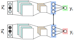
Check the figure above. The blue layer is the hidden layer used for generating the embedding, whose output is represented by $h_{\theta}(X_i)$. $y$ is the final output. If $X_i$ and $X_j$ are close-by, the distance between them is represented by $d(h_{\theta}(X_i), h_{\theta}(X_j))$.
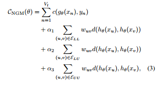
The cost-function is below. Don’t let this scare you. The first term is just the total loss from the predictions of the network for labeled data. The next three terms are for tweaking the importance of distances between the various (labeled / unlabeled) -(labeled / unlabeled) pairs, weighed by their respective edge weights, $w_{uv}$.
I skimmed through the paper to get the gist, but I wonder that the core contribution of such a network is to go from a graph-based structure to an embedding. If we were to construct an embedding directly from the graph structure, and train a NN separately using the embedding as the input, my guess is it should fetch similar results with a less complex objective function.
Read moreA Gentle Intro to PyTorch
24 Apr 2017 - 3 minute read
PyTorch is a fairly new deep-learning framework released by Facebook, which reminds me of the JS framework frenzy. But having played around with PyTorch a slight bit, it already feels fun.
To keep things short, I liked it because:
- Unlike TensorFlow it allows me to easily print Tensors on the screen (no seriously, this is a big deal for me since I usually take several iterations to get a DL implementation right).
- TensorFlow adds a layer between Python and TensorFlow. TensorFlow even has it’s own variable scope. This is way too much abstraction, that I don’t appreciate for my experimental interests.
- Interop with numpy is easy in PyTorch, with the simple
.numpy()suffix to convert a Tensor to a numpy array. - Unlike Torch, it is not in Lua (also doesn’t need the LuaRocks package manager).
- Unlike Caffe2, I don’t have to write C++ code and write build scripts.
PyTorch’s website has a 60 min. blitz tutorial, which is laid out pretty well.
Here is the summary to get you started on PyTorch:
torch.Tensoris yournp.array(the NumPy array).torch.Tensor(3,4)will create aTensorof shape (3,4).- All the functions are pretty standard. Such as
torch.randcan be used to generate random Tensors. - Indexing in Tensors is pretty similar to NumPy as well.
.numpy()allows converting Tensor to a numpy array.- For the purpose of a compute graph, PyTorch lets you create
Variables which are similar toplaceholderin TF. - Creating a compute graph and computing the gradient is pretty easy (and automatic).
This is all it takes to compute the gradient, where x is a variable:
x = Variable(torch.ones(2, 2), requires_grad=True)
y = x + 2
z = y * y * 3
out = z.mean()

out.backward()
print(x.grad)
Doing backprop simply with the backward method call on the scalar out, computes gradients all the way to x. This is amazing!
- For NN, there is an
nn.Modulewhich wraps around the boring boiler-plate. - A simple NN implementation is below for solving the MNIST dataset, instead of the CIFAR-10 dataset that the tutorial solves:
import torch.nn.functional as F

class Net(nn.Module):
    def __init__(self):
        super(Net, self).__init__()
        self.conv1 = nn.Conv2d(1, 1, 5)
        self.conv2 = nn.Conv2d(1, 1, 5)
        self.pool = nn.MaxPool2d(2, 2)
        self.fc1 = nn.Linear(1 * 10 * 10, 100)
        self.fc2 = nn.Linear(100, 10)

    def forward(self, x):
        x = F.relu((self.conv1(x)))
        x = F.relu(F.max_pool2d((self.conv2(x)), 2))
        x = x.view(-1, 1 * 10 * 10)
        x = F.relu(self.fc1(x))
        x = F.relu(self.fc2(x))
        return F.log_softmax(x)
As seen, in the __init__ method, we just need to define the various NN layers we are going to be using. Then the forward method just runs through them. The view method is analogous to the NumPy reshape method.
The gradients will be applied after the backward pass, which is auto-computed. The code is self-explanatory and fairly easy to understand.
- Torch also keeps track of how to retrieve standard data-sets such as CIFAR-10, MNIST, etc.
- After getting the data, from the data-loader you can proceed to play with it. Below are rest of the pieces required to complete the implementation (almost all of it is from the tutorial):
# Create the net and define the optimization criterion
net = Net()
# The loss function
criterion = nn.CrossEntropyLoss()
# Which optimization technique will you apply?
optimizer = optim.SGD(net.parameters(), lr=0.001, momentum=0.5)

# zero the parameter gradients
optimizer.zero_grad()

for epoch in range(20):  # loop over the dataset multiple times
    # Run per epoch
    running_loss = 0.0
    for i, data in enumerate(trainloader, 0):
        # get the inputs
        inputs, labels = data

        # wrap them in Variable
        inputs, labels = Variable(inputs), Variable(labels)

        # zero the parameter gradients
        optimizer.zero_grad()

        # Forward Pass
        outputs = net(inputs)
        # Compute loss function
        loss = criterion(outputs, labels)
        # Backward pass and gradient update
        loss.backward()
        optimizer.step()
The criterion object is used to compute your loss function. optim has a bunch of convex optimization algorithms such as vanilla SGD, Adam, etc. As promised, simply calling the backward method on the loss object allows computing the gradient.
- Assuming you are working on the tutorial. Try to solve the tutorial for MNIST data instead of CIFAR-10.
- Instead of the 3-channel (RGB) image of size 24x24 pixels, the MNIST images are single channel 28x28 pixel images.
Overall, I could get to 96% accuracy, with the current setup. The complete gist is here.
Read moreBack to Basics: Linear Regression
05 Apr 2017 - 6 minute read
Taking inspiration from Werner Vogel’s ‘Back to Basics’ blogposts, here is one of my own posts about fundamental topics. While on a long-haul flight with no internet connectivity, having exhausted the books on my kindle, and hardly any inflight-entertainment, I decided to code up Linear Regression in Python. Let’s look at both the theory and implementation of the same.
Theory
Essentially, in Linear Regression, we try to estimate a dependent variable $y$, using independent variables $x_1$, $x_2$, $x_3$, $…$, using a linear model.
More formally,
\[y = b + W_1 x_1 + W_2 x_2 + ... + W_n x_n + \epsilon\]Where, $W$ is the weight vector, $b$ is the bias term, and $\epsilon$ is the noise in the data.
It can be used when there is a linear relationship between the input $X$ (input vector containing all the $x_i$, and $y$).
One example could be, given a vending machine’s sales of different kind of soda, predict the total profit made. Let’s say there are three kinds of soda, and for each can of that variety sold, the profit is 0.25, 0.15 and 0.20 respectively. Also, we know that there will be a fixed cost in terms of electricity and maintenance for the machine, this will be our bias, and it will be negative. Let’s say it is $100. Hence, our profit will be:
\[y = -100 + 0.25x_1 + 0.15x_2 + 0.20x_3\]The problem is usually the inverse of the above example. Given the profits made by the vending machine, and sales of different kinds of soda (i.e., several pairs of $(X_i, y_i)$), find the above equation. Which would mean being able to find $b$, and $W$. There is a closed-form solution for Linear Regression, but it is expensive to compute, especially when the number of variables is large (10s of thousands).
Generally in Machine Learning the following approach is taken for similar problems:
- Make a guess for the parameters ($b$ and $W$ in our case).
- Compute some sort of a loss function. Which tells you how far you are from the ideal state.
- Find how much you should tweak your parameters to reduce your loss.
Step 1 The first step is fairly easy, we just pick a random $W$ and $b$. Let’s say $\theta = (W, b)$, then $h_\theta(X_i) = b + X_i.W$. Given an $X_i$, our prediction would be $h_\theta(X_i)$.
Step 2 For the second step, one loss function could be, the average absolute difference between the prediction and the real output. This is called the ‘L1 norm’.
\[L_1 = \frac{1}{n}\sum_{i=1}^{n} \text{abs}(h_\theta(X_i) - y_i)\]L1 norm is pretty good, but for our case, we will use the average of the squared difference between the prediction and the real output. This is called the ‘L2 norm’, and is usually preferred over L1.
\[L_2 = \frac{1}{2n}\sum_{i=1}^{n} (h_\theta(X_i) - y_i)^2\]Step 3 We have two sets of params $b$ and $W$. Ideally, we want $L_2$ to be 0. But that would depend on the choices of these params. Initially the params are randomly chosen, but we need to tweak them so that we can minimize $L_2$.
For this, we follow the Stochastic Gradient Descent algorithm. We will compute ‘partial derivatives’ / gradient of $L_2$ with respect to each of the parameters. This will tell us the slope of the function, and using this gradient, we can adjust these params to reduce the value of the method.
Again,
$L_2 = \frac{1}{2n}\sum_{i=1}^{n} (h_\theta(X_i) - y_i)^2$.
Deriving w.r.t. $b$ and applying chain rule,
$\large \frac{\partial L}{\partial b}$ = $2 . \large\frac{1}{2n}$ $\sum_{i=1}^{n} (h_\theta(X_i) - y_i) . 1$ (Since, $\frac{\partial (h_\theta(X_i) - y_i)}{\partial b} = 1$)
$ \implies \large \frac{\partial L}{\partial b}$ $= \sum_{i=1}^{n} (h_\theta(X_i) - y_i)$
Similarly, deriving w.r.t. $W_j$ and applying chain rule,
$\large \frac{\partial L}{\partial W_j}$ = $\large\frac{1}{n}$ $\sum_{i=1}^{n} (h_\theta(X_i) - y_i) . X_{ij}$
Hence, at each iteration, the updates we will perform will be,
$b = b - \eta \large\frac{\partial L}{\partial b}$, and, $W_j = W_j - \eta \large\frac{\partial L}{\partial W_j}$.
Where, $\eta$ is what is called the ‘learning rate’, which dictates how big of an update we will make. If we choose this to be to be small, we would make very small updates. If we set it to be a large value, then we might skip over the local minima. There are a lot of variants of SGD with different tweaks around how we make the above updates.
Eventually we should converge to a value of $L_2$, where the gradients will be nearly 0.
Implementation
The complete implementation with dummy data in about 100 lines is here. A short walkthrough is below.
The only two libraries that we use are numpy (for vector operations) and matplotlib (for plotting losses). We generate random data without any noise.
def linear_sum(X, W, b):
    return X.dot(W) + b

def data_gen(num_rows, num_feats, op_gen_fn=linear_sum):
    data = {}
    W = 0.1 * np.random.randn(num_feats)
    b = 0.1 * np.random.randn()
    data['X'] = np.random.randn(num_rows, num_feats)
    data['y'] = op_gen_fn(data['X'], W, b)
    return data
Where num_rows is $n$ as used in the above notation, and num_feats is the number of variables. We define the class LinearRegression, where we initialize W and b randomly initially. Also, the predict method computes $h_\theta(X)$.
class LinearRegression(object):
    def __init__(self):
        self.W = None
        self.b = 0

    def init_matrix(self, X):
        self.W = 0.1 * np.random.randn(X.shape[1])
        self.b = 0.1 * np.random.randn()

    def predict(self, X):
        if self.W is None:
            self.init_matrix(X)

        return X.dot(self.W) + self.b
The crux of the code is in the train method, where we compute the gradients.
def train(self, data, iters, lr):
        X = data['X']
        y = data['y']

        orig_pred = self.predict(X)
        orig_l1 = self.l1_loss(orig_pred, y)
        orig_l2 = self.l2_loss(orig_pred, y)

        l1 = orig_l1
        l2 = orig_l2

        l1_losses = []
        l2_losses = []
        l1_losses.append(l1)
        l2_losses.append(l2)

        for it in range(iters):
            pred = self.predict(X)

            # Computing gradients
            s1 = (pred - y)
            s2 = np.multiply(X, np.repeat(s1, X.shape[1])\
                    .reshape(X.shape[0], X.shape[1]))
            wGrad = np.sum(s2, axis=0) / X.shape[0]
            bGrad = np.sum(s1) * 1.0 / X.shape[0]

            # Updates to W and b
            wDelta = -lr * wGrad
            bDelta = -lr * bGrad
            self.W += wDelta
            self.b += bDelta

            l1 = self.l1_loss(pred, y)
            l2 = self.l2_loss(pred, y)

            l1_losses.append(l1)
            l2_losses.append(l2)

        print 'Original L1 loss: %Lf, L2 loss: %Lf ' % (orig_l1, orig_l2)
        print 'Final L1 loss: %Lf, L2 loss: %Lf' % (l1, l2)
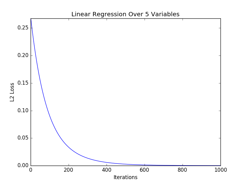
For the given input, with the fixed seed and five input variables, the solution as per the code is:
- b:  -0.081910978042
- W:  [-0.04354505  0.00196225 -0.2143796   0.1617485  -0.17349839]
This is how the $L_2$ loss converges over number of iterations:
To verify that this is actually correct, I serialized the input to a CSV file and used R to solve this.
> df <- read.delim(file="lin_reg_data", header=F, sep=",")
> lm(df[,1] ~ df[,2]+df[,3]+df[,4]+df[,5]+df[,6])

Call:
lm(formula = df[, 1] ~ df[, 2] + df[, 3] + df[, 4] + df[, 5] +
    df[, 6])

Coefficients:
(Intercept)      df[, 2]      df[, 3]      df[, 4]      df[, 5]      df[, 6]
  -0.084175    -0.041676    -0.005627    -0.213620     0.164027    -0.179344
The intercept is same as $b$, and the rest five outputs are the $W_i$, and are similar to what my code found.