Semi-Supervised Learning is useful in scenarios where you have some labeled data, and lots of unlabeled data. If there is a way to cluster together training examples by a measure of similarity, and we can assume that examples close to each other in these clusterings are likely to have the same labels, then Semi-Supervised Learning can be pretty useful.

Essentially the premise is that labeling all the data is expensive, and we should learn as much as we can from as small a dataset as possible. For their data-labeling needs, the industry either relies on Mechanical Turks or full-time labelers on contract (Google Search is one example where they have a large team of human raters). Overall, it is costly to build a large labeled dataset. Therefore, if we can minimize our dependence on labeled data, and learn from known / inferred similarity within the dataset, that would be great. That’s where Semi-Supervised Learning helps.

Assume there is a graph-structure to our data, where a node is a datum / row, which needs to be labeled. And an edge exists between two nodes if they are similar, along with a weight. In this case, Label Propagation is a classic technique which has been used commonly.

I read this paper from Google Research which does a good job of generalizing and summarizing similar work done by Weston et. al, 2012, around training Neural Nets augmented by such a graph-based structure.

To summarize the work very quickly, the network tries to do two things:

a. For labeled data, try to predict the correct label (of course),

b. For the entire data set, try to learn a representation of each datum (embedding) in the hidden layers of the neural net.

For nodes which are adjacent to each other, the distance between their respective embeddings should be small, and the importance of keeping this distance small is proportional to the edge weight. That is, if there are two adjacent nodes with a high edge weight, if the neural net doesn’t learn to create embeddings such that these two examples are close to each other, there would be a larger penalty, than if the distance was smaller / the edge weight was lower.

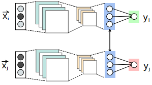
Check the figure above. The blue layer is the hidden layer used for generating the embedding, whose output is represented by $h_{\theta}(X_i)$. $y$ is the final output. If $X_i$ and $X_j$ are close-by, the distance between them is represented by $d(h_{\theta}(X_i), h_{\theta}(X_j))$.

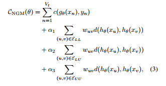
The cost-function is below. Don’t let this scare you. The first term is just the total loss from the predictions of the network for labeled data. The next three terms are for tweaking the importance of distances between the various (labeled / unlabeled) -(labeled / unlabeled) pairs, weighed by their respective edge weights, $w_{uv}$.

I skimmed through the paper to get the gist, but I wonder that the core contribution of such a network is to go from a graph-based structure to an embedding. If we were to construct an embedding directly from the graph structure, and train a NN separately using the embedding as the input, my guess is it should fetch similar results with a less complex objective function.