Modulo a Large Prime: Why?

Feb 4th, 2017 | Comments

The Karp-Rabin algorithm for string matching (which is pretty elegant, and I strongly prefer it to KMP in most settings), uses the modulo operator when computing the hash of the strings. What is interesting is, it recommends using a prime number as the modulus for doing this.

Similarly, when computing which hash-table bucket a particular item goes to, the common way to do it is: $b = h(x)\bmod n$. Where $h(x)$ is the hash function output, $n$ is the number of buckets you have.

Why do we need a prime modulus?

In hash functions, one should expect to receive pathological inputs. Assume, $n = 8$. What happens, if we receive $h(x)$ such as that they are all multiples of $4$? That is, $h(x)$ is in $[4, 8, 12, 16, 20, …]$, which in $\bmod 8$ arithmetic will be $[4, 0, 4, 0, 4, …]$. Clearly, only 2 buckets will be used, and the rest 6 buckets will be empty, if the input follows this pattern. There are several such examples.

As a generalization, if the greatest common factor of $h(x)$ and $n$ is $g$, and the input is going to be of the form $[h(x), 2h(x), 3h(x), …]$, then the number of buckets that will be used is $\large \frac{n}{g}$. This is easily workable on paper.

We ideally want to be able to use all the buckets. Hence, the number of buckets used, $\large \frac{n}{g}$ $= n$, which implies $g = 1$.

This means, the input and the modulus ($n$) should be co-prime (i.e., share no common factors). Given, we can’t change the input, we can only change the modulus. So we should choose the modulus such that it is co-prime to the input.

For the co-prime requirement to hold for all inputs, $n$ has to be a prime. Now it will have no common factors with any input (except it’s own multiples), and $g$ would be 1.

Therefore, we need the modulus to be prime in such settings.

Let me know if I missed out on something, or my intuition here is incorrect.

A Gentle Intro to Recurrent Neural Networks in TensorFlow

Jan 12th, 2017 | Comments

Recurrent Neural Networks are pretty interesting. Please read Andrej Karpathy’s post about their effectiveness here, if you haven’t already. I am not going to cover a lot of new material in the post, but mostly drawing inspiration from his min-char-rnn and R2RT’s post about RNNs, and giving a gentle intro to using TF to write a simple RNN.

I picked TensorFlow rather than Caffe, because of the possibility of being able to run my code on mobile, which I enjoy. Also, the documentation and community around TF seemed slightly more vibrant than Caffe/Caffe2.

What we want to do is:

Feed the RNN some input text, one character at a time.
Train the RNN to predict the next character.
The RNN keeps a hidden state (some sort of context), it should be able to learn to predict the next character accurately.
Try to do it without using the fancy stuff as much as possible.

Quick Intro

The hidden state at time step $t$ is $h_t$ is a function of the hidden step at the previous time-step, and the current input. Which is:

$h_t = f_W(h_{t-1}, x_t)$

$f_W$ can be expanded to:

$h_t = \tanh(W_{xh}x_{t} + W_{hh}h_{t-1})$

$W_{xh}$ is a matrix of weights for the input at that time $x_t$. $W_{hh}$ is a matrix of weights for the hidden-state at the previous time-step, $h_{t-1}$.

Finally, $y_{t}$, the output at time-step $t$ is computed as:

$y_{t} = W_{hy}h_{t}$

Dimensions:

For those like me who are finicky about dimensions:

Assuming input $x_t$ is of size $V \times N$. Where $V$ is the size of one example, and there are $N$ examples.
Our hidden state per example is of size $H$, so $h_i$ is of size $H \times N$ for all $N$ examples.
Easy to infer then is $W_{xh}$ is of size $H \times V$, $W_{hh}$ is of size $H \times H$.
$y_t$ has to be of size $V \times N$, hence $W_{hy}$ is of size $V \times H$

Code Walkthrough

This is my implementation of min-char-rnn, which I am going to use for the purpose of the post.

We start with just reading the input data, finding the distinct characters in the vocabulary, and associating an integer value with each character. Pretty standard stuff.

data = open('input.txt', 'r').read()
chars = list(set(data))
data_size, vocab_size = len(data), len(chars)
print 'data has %d characters, %d unique.' % (data_size, vocab_size)

char_to_ix = { ch:i for i,ch in enumerate(chars) }
ix_to_char = { i:ch for i,ch in enumerate(chars) }

# Convert an array of chars to array of vocab indices
def c2i(inp):
    return map(lambda c:char_to_ix[c], inp)

def i2c(inp):
    return map(lambda c:ix_to_char[c], inp)

Then we specify our hyperparameters, such as size of the hidden state ($H$). seq_length is the number of steps we will train an RNN per initialization of the hidden state. In other words, this is the maximum context the RNN is expected to retain while training.

# hyperparameters
hidden_size = 100 # size of hidden layer of neurons
seq_length = 25 # number of steps to unroll the RNN for
learning_rate = 2e-1
batch_size = 50
num_epochs = 500

We have a method called genEpochData which does nothing fancy, apart from breaking the data into batch_size number of batches, each with a fixed number of examples, where each example has an (x, y) pair, both of which are of seq_length length. x is the input, and y is the output.

In our current setup, we are training the network to predict the next character. So y would be nothing but x shifted right by one character.

Now that we have got the boiler-plate out of the way, comes the fun part.

Light-Weight Intro to TensorFlow

The way TensorFlow (TF) works is that it creates a computational graph. With numpy, I was used to creating variables which hold actual values. So data and computation went hand-in-hand.

In TF, you define ‘placeholders’, which are where your input will go, such as place holders for x and y, like so:

# Input
x = tf.placeholder(tf.int32, shape=(seq_length), name="x")
y = tf.placeholder(tf.int32, shape=(seq_length), name="y")

Then you can define ‘operations’ on these input placeholders. In the code below, we convert x and y to their respective ‘one hot’ representations (a binary vector of size, vocab_size, where the if the value of x is i, the i-th bit is set).

# One Hot representation of the input
x_oh = tf.one_hot(indices=x, depth=vocab_size)
y_oh = tf.one_hot(indices=y, depth=vocab_size)

This is a very simple computation graph, wherein if we set the placeholders correctly, x_oh and y_oh will have the corresponding one-hot representations of the x and y. But you can’t print out their values directly, because they don’t contain them. We need to evaluate them through a TF session (coming up later in the post).

One can also define variables, such as when defining the hidden state, we do it this way:

state = tf.zeros([hidden_size, 1])

We’ll use the above declared variable and placeholders to compute the next hidden state, and you can compute arbitrarily complex functions this way. For example, the picture below from the TF whitepaper shows how can we represent the output of a Feedforward NN using TF (b and W are variables, and x is the placeholder. Everything else is an operation).

Computation Graph in TF

Simple RNN using TF

The code below computes $y_t$, given the $x_t$ and $h_{t-1}$.

# Actual math behind computing the output and the next state of the RNN.
def rnn_cell(rnn_input, cur_state):
    # variable_scope helps define variables in a namespace.
    with tf.variable_scope('rnn_cell', reuse=True):
        Wxh = tf.get_variable('Wxh', [hidden_size, vocab_size])
        Whh = tf.get_variable('Whh', [hidden_size, hidden_size])
        Why = tf.get_variable('Why', [vocab_size, hidden_size])
        bh = tf.get_variable('bh', [hidden_size, 1])
        by = tf.get_variable('by', [vocab_size, 1])

    # expand_dims is required to make the input a 2-D tensor.
    inp = tf.expand_dims(rnn_input, 1)

    next_state = tf.tanh(tf.matmul(Wxh, inp) + tf.matmul(Whh, cur_state) + bh)
    y_hat = tf.matmul(Why, next_state) + by
    return y_hat, next_state

Now we are ready to complete our computation graph.

# Convert the VxN tensor into N tensors of Vx1 size each.
rnn_inputs = tf.unpack(x_oh)
rnn_targets = tf.unpack(y_oh)

logits = []
# Iterate over all the input vectors
for rnn_input in rnn_inputs:
    y_hat, state = rnn_cell(rnn_input, state)
    # Convert y_hat into a 1-D tensor
    y_hat = tf.squeeze(y_hat)
    logits.append(y_hat)

# Use the helper method to compute the softmax losses
# (It basically compares the outputs to the expected output)
losses = [tf.nn.softmax_cross_entropy_with_logits(logit, target) for logit, target in zip(logits, rnn_targets)]
# Compute the average loss over the batch
total_loss = tf.reduce_mean(losses)

As we saw above, we can compute the total loss in the batch pretty easily. This is usually the easier part.

While doing CS231N assignments, I learned the harder part was the back-prop, which is based on how off your predictions are from the expected output.You need to compute the gradients at each stage of the computation graph. With large computation graphs, this is tedious and error prone. What a relief it is, that TF does it for you automagically (although it is super to know how backprop really works).

# Under the hood, the operation below computes the gradients and does the backprop!
train_step = tf.train.AdadeltaOptimizer(learning_rate).minimize(total_loss)

Evaluating the graph

Evaluating the graph is pretty simple too. You need to initialize a session, and then initialize all the variables. The run method of the Session object does the execution of the graph. The first input is the list of the graph nodes that you want to evaluate. The second argument is the dictionary of all the placeholders.

It returns you the list of values for each of the requested nodes in order.

with tf.Session() as sess:
  sess.run(tf.initialize_all_variables())

  # <Add code to generate epoch data>
  # Assuming x_i and y_i have the input and output for the batch:
    loss, tloss, _, logits_, rnn_targets_, epoch_state = \
        sess.run([losses, total_loss, train_step, logits,
                  rnn_targets, state], \
                  feed_dict={x:x_i, y:y_i, init_state:epoch_state}
                )

After this, it is pretty easy to stitch all this together into a proper RNN.

Results

While writing the post, I discovered a couple of implementation issues, which I plan to fix. But nevertheless, training on a Shakespeare’s ‘The Tempest’, after a few hundred epochs, the RNN generated this somewhat english-like sample:

SEBASTIAN.
And his leainstsunzasS!

FERDINAND.
I lost, and sprery
RS]
How it ant thim hand

Not too bad. It learns that there are characters named Sebastian and Ferdinand. And mind you this was a character level model, so this isn’t super crappy :-)

(All training was done on my MBP. No NVidia GPUs were used whatsoever. I have a good ATI Radeon GPU at home, but TF doesn’t support OpenCL yet. It’s coming soon-ish though.)

Systems Design: Facebook TAO

Dec 29th, 2016 | Comments

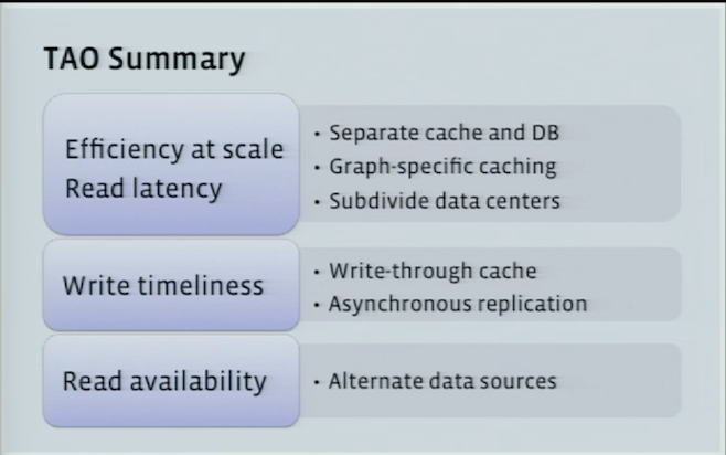
TAO is a very important part of the infrastructure at Facebook. This is my attempt at summarizing the TAO paper, and the blog post, and the talk by Nathan Bronson. I am purely referring to public domain materials for this post.

Motivation

Memcache was being used as a cache for serving the FB graph, which is persisted on MySQL. Using Memcache along with MySQL as a look-aside/write-through cache makes it complicated for Product Engineers to write code modifying the graph while taking care of consistency, retries, etc. There has to be glue code to unify this, which can be buggy.

A new abstraction of Objects & Associations was created, which allowed expressing a lot of actions on FB as objects and their associations. Initially there seems to have been a PHP layer which deprecated direct access to MySQL for operations which fit this abstraction, while continuing to use Memcache and MySQL underneath the covers.

This PHP layer for the above model is not ideal, since:

Incremental Updates: For one-to-many associations, such as the association between a page and it’s fans on FB, any incremental update to the fan list, would invalidate the entire list in the cache.
Distributed Control Logic: Control logic resides in fat clients. Which is always problematic.
Expensive Read After Write Consistency: Unclear to me.

TAO

TAO is a write-through cache backed by MySQL.

TAO objects have a type ($otype$), along with a 64-bit globally unique id. Associations have a type ($atype$), and a creation timestamp. Two objects can have only one association of the same type. As an example, users can be Objects and their friendship can be represented as an association. TAO also provides the option to add inverse-assocs, when adding an assoc.

Objects-Assocs in TAO

API

The TAO API is simple by design. Most are intuitive to understand.

assoc_add(id1, atype, id2, time, (k→v)*): Add an association of type atype from id1 to id2.
assoc_delete(id1, atype, id2): Delete the association of type atype from id1 to id2.
assoc_get(id1, atype, id2set, high?, low?): Returns assocs of atype between id1 and members of id2set, and creation time lies between $[high, low]$.
assoc_count(id1, atype): Number of assocs from id1 of type atype.
And a few others, refer to the paper.

As per the paper:

TAO enforces a per-atype upper bound (typically 6,000) on the actual limit used for an association query.

This is also probably why the maximum number of friends you can have on FB is 5000.

Architecture

There are two important factors in the TAO architecture design:

On FB the aggregate consumption of content (reads), is far more than the aggregate content creation (writes).
The TAO API is such that, to generate a newsfeed story (for example), the web-server will need to do the dependency resolution on its own, and hence will require multiple round-trips to the TAO backend. This further amplifies reads as compared to writes, bringing the read-write ratio to 500:1, as mentioned in Nathan’s talk.

The choice of being okay with multiple round-trips to build a page, while wanting to ensure a snappy product experience, imposes the requirement that:

Each of these read requests should have a low read latency (cannot cross data-center boundaries for every request).
The read availability is required to be pretty high.

Choice of Backing Store

The underlying DB is MySQL, and the TAO API is mapped to simple SQL queries. MySQL had been operated at FB for a long time, and internally backups, bulk imports, async replication etc. using MySQL was well understood. Also MySQL provides atomic write transactions, and few latency outliers.

Sharding / Data Distribution

Objects and Associations are in different tables. Data is divided into logical shards. Each shard is served by a database.

Quoting from the paper:

In practice, the number of shards far exceeds the number of servers; we tune the shard to server mapping to balance load across different hosts.

And it seems like the sharding trick we credited to Pinterest might have been used by FB first :-)

Each object id contains an embedded shard id that identifies its hosting shard.

The above setup means that your shard id is pre-decided. An assoc is stored in the shard belonging to its id1.

Consistency Semantics

TAO also requires “read-what-you-wrote” consistency semantics for writers, and eventual consistency otherwise.

Leader-Follower Architecture

TAO is setup with multiple regions, and user requests hit the regions closest to them. The diagram below illustrates the caching architecture. TAO Leader-Follower Setup

There is one ‘leader’ region and several ‘slave’ regions. Each region has a complete copy of the databases. There is an ongoing async replication between leader to slave(s). In each region, there are a group of machines which are ‘followers’, where each individual group of followers, caches and completely serves read requests for the entire domain of the data. Clients are sticky to a specific group of followers.

In each region, there is a group of leaders, where there is one leader for each shard. Read requests are served by the followers, cache misses are forwarded to the leaders, which in turn return the result from either their cache, or query the DB.

Write requests are forwarded to the leader of that region. If the current region is a slave region, the request is forwarded to the leader of that shard in the master region.

The leader sends cache-refill/invalidation messages to its followers, and to the slave leader, if the leader belongs to the master region. These messages are idempotent.

The way this is setup, the reads can never be stale in the master leader region. Followers in the master region, slave leader and by extension slave followers might be stale as well. The authors mention an average replication lag of 1s between master and slave DBs, though they don’t mention whether this is same-coast / cross-country / trans-atlantic replication.

When the leader fails, the reads go directly to the DB. The writes to the failed leader go through a random member in the leader tier.

Read Availability

There are multiple places to read, which increases read-availability. If the follower that the client is talking to, dies, the client can talk to some other follower in the same region. If all followers are down, you can talk directly to the leader in the region. Following whose failure, the client contacts the DB in the current region or other followers / leaders in other regions.

Read Availability in TAO

Performance

These are some client-side observed latency and hit-rate numbers in the paper.